Markov Decision Processes
The Markov decision process is a model of predicting outcomes under uncertainty.It is one way to optimize your actions to find the best outcome in spite of the random element from the environment.
Expressing a problem as an MDP is the first step towards solving it through techniques like dynamic programming or other techniques of RL.
Markov Decision Processes (MDPs) are stochastic processesthat exhibit the Markov Property. The Markov Property is used to refer to situations where the probabilities of different outcomes are not dependent on past states: the current state is all you need to know. This property is sometimes called “memorylessness”. [3]
To express a problem using MDP, one needs to define the followings
states of the environment
actions the agent can take on each state
rewards obtained after taking an action on a given state
state transition probabilities

Once the problem is expressed as an MDP, one can use dynamic programming or many other techniques to find the optimum policy. [2]
The problem of k-armed bandits problem is that it only considers short-term returns while in many cases long-term thinking is needed in order to optimize rewards.Markov decision processes (MDPs) are a classical formalization of sequential decision making, where actions influence not just immediate rewards, but also subsequent situations, or states, and through those future rewards.
Three major parties involved in MDPs are:
- agent: the learner and decision maker
- environment: the thing the agent interacts with, comprising everything outside the agent
-
reward: numerical values that the agent seeks to maximize over time through its choice of actions, it passed from the environment to the agent

Typical agent and environment interaction in MPDs can be described as above. The agent and environment interact at each of a sequence of discrete time steps, t = 0, 1, 2, 3…. Note that the real time interval between each time step can be anything depending on the specific problem. At time step t, the agent select an action At based on its environment’s state St. Such an action will bring reward Rt+1 to the environment and change its state from St to St+1. The MDP and agent thereby give rise to a trajectory like this: S0, A0, R1, S1, A1, R2, S2, A2, R3, …
The dynamics of a finite MDP which has finite number of states, actions and rewards is defined as the function p as follows:

Importantly, the following condition is satisfied.
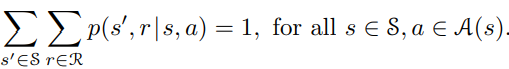
The essence of this equation is that the probability of each possible value for St and Rt depends only on the immediately preceding state and action, St-1 and At-1, irrelevant of earlier states and actions. That is to say, the present state have the Markov property — it includes all the information necessary to predict the future interactions.
Previously we mentioned that MDPs considers long-term rewards while k-armed bandits problem only considers immediate reward. Why do we care about reward? Because it is what we are trying to optimize in reinforcement learning. A formal definition as the reward hypothesis is the goals and purposes of reinforcement learning is to maximize the expected value of the cumulative sum of a received reward.
So how do we define rewards mathematically?
There are two types of tasks: episodic task and continuous task. Episodic tasks are tasks in which the interaction breaks natually into subsequences called episodes, each episode ends in a terminal state, and episodes are independent. Continous tasks are tasks in which the interactions goes on continually and no terminal state exist.
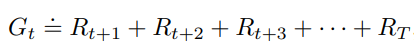
For episodic task, we seek to maximize expected return. Here expected return instead of return is used because of randomness involved in the process. The return is the sum of rewards:
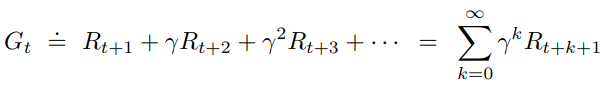
For continous task, the above equation easily goes into infinity. A mathematical trick is to introduce discounting by adding discount rate gama ([0, 1]) into future rewards as follows:
Mathematically, we can prove Gt is finite.

If gama < 1 and the reward is a constant +1, then the return is

The discount rate indicates a reward received k time steps in the future is worth only gama^(k-1) times what it would be worth if it were received immediately. If gama = 0, it means the agent only cares about the immediate reward. The closer gama to 1, the stronger the agent takes future rewards into account.
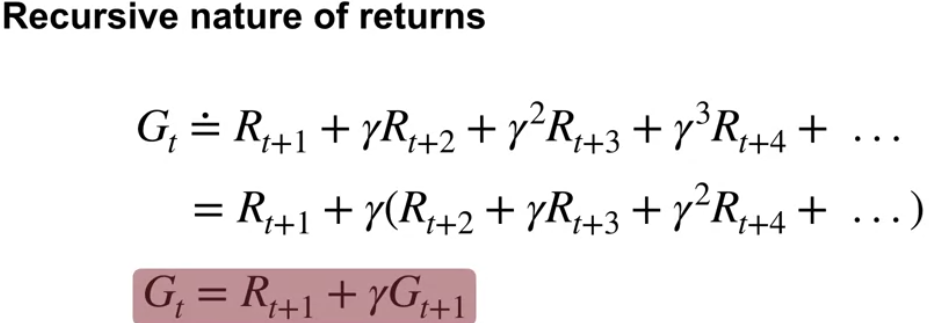
Alternatively, Gt can be defined recursively to allow us calculate Gt backwards starting from the termination state G(T) = 0.
The probability distribution of taking actions At from a state St is called policy π(At
St). The goal of solving an MDP is to find an optimal policy.
References:
-
https://towardsdatascience.com/real-world-applications-of-markov-decision-process-mdp-a39685546026 (real-world examples)
-
https://web.stanford.edu/group/sisl/k12/optimization/MO-unit5-pdfs/5.9MDPs.pdf
Note: This article is part of my personal note series of the Reinforcement learning Specialization provided by the Unversity of Alberta and Alberta Machine Intelligence Institute on Coursera.
Markov Decision Processes
The Markov decision process is a model of predicting outcomes under uncertainty.It is one way to optimize your actions to find the best outcome in spite of the random element from the environment.
Expressing a problem as an MDP is the first step towards solving it through techniques like dynamic programming or other techniques of RL.
Markov Decision Processes (MDPs) are stochastic processesthat exhibit the Markov Property. The Markov Property is used to refer to situations where the probabilities of different outcomes are not dependent on past states: the current state is all you need to know. This property is sometimes called “memorylessness”. [3]
To express a problem using MDP, one needs to define the followings
states of the environment
actions the agent can take on each state
rewards obtained after taking an action on a given state
state transition probabilities
Once the problem is expressed as an MDP, one can use dynamic programming or many other techniques to find the optimum policy. [2]
The problem of k-armed bandits problem is that it only considers short-term returns while in many cases long-term thinking is needed in order to optimize rewards.Markov decision processes (MDPs) are a classical formalization of sequential decision making, where actions influence not just immediate rewards, but also subsequent situations, or states, and through those future rewards.
Three major parties involved in MDPs are:
- agent: the learner and decision maker
- environment: the thing the agent interacts with, comprising everything outside the agent
-
reward: numerical values that the agent seeks to maximize over time through its choice of actions, it passed from the environment to the agent
Typical agent and environment interaction in MPDs can be described as above. The agent and environment interact at each of a sequence of discrete time steps, t = 0, 1, 2, 3…. Note that the real time interval between each time step can be anything depending on the specific problem. At time step t, the agent select an action At based on its environment’s state St. Such an action will bring reward Rt+1 to the environment and change its state from St to St+1. The MDP and agent thereby give rise to a trajectory like this: S0, A0, R1, S1, A1, R2, S2, A2, R3, …
The dynamics of a finite MDP which has finite number of states, actions and rewards is defined as the function p as follows:
Importantly, the following condition is satisfied.
The essence of this equation is that the probability of each possible value for St and Rt depends only on the immediately preceding state and action, St-1 and At-1, irrelevant of earlier states and actions. That is to say, the present state have the Markov property — it includes all the information necessary to predict the future interactions.
Previously we mentioned that MDPs considers long-term rewards while k-armed bandits problem only considers immediate reward. Why do we care about reward? Because it is what we are trying to optimize in reinforcement learning. A formal definition as the reward hypothesis is the goals and purposes of reinforcement learning is to maximize the expected value of the cumulative sum of a received reward.
So how do we define rewards mathematically?
There are two types of tasks: episodic task and continuous task. Episodic tasks are tasks in which the interaction breaks natually into subsequences called episodes, each episode ends in a terminal state, and episodes are independent. Continous tasks are tasks in which the interactions goes on continually and no terminal state exist.
For episodic task, we seek to maximize expected return. Here expected return instead of return is used because of randomness involved in the process. The return is the sum of rewards:
For continous task, the above equation easily goes into infinity. A mathematical trick is to introduce discounting by adding discount rate gama ([0, 1]) into future rewards as follows:
Mathematically, we can prove Gt is finite.
If gama < 1 and the reward is a constant +1, then the return is
The discount rate indicates a reward received k time steps in the future is worth only gama^(k-1) times what it would be worth if it were received immediately. If gama = 0, it means the agent only cares about the immediate reward. The closer gama to 1, the stronger the agent takes future rewards into account.
Alternatively, Gt can be defined recursively to allow us calculate Gt backwards starting from the termination state G(T) = 0.
| The probability distribution of taking actions At from a state St is called policy π(At | St). The goal of solving an MDP is to find an optimal policy. |
References:
-
https://towardsdatascience.com/real-world-applications-of-markov-decision-process-mdp-a39685546026 (real-world examples)
-
https://web.stanford.edu/group/sisl/k12/optimization/MO-unit5-pdfs/5.9MDPs.pdf
Note: This article is part of my personal note series of the Reinforcement learning Specialization provided by the Unversity of Alberta and Alberta Machine Intelligence Institute on Coursera.
Comments
Join the discussion for this article on this ticket. Comments appear on this page instantly.