K-armed Bandit Problem
K-armed bandit problem (or multi-armed bandit problem) is a problem in which a fixed limited set of resources must be allocated between competing or alternative choices in a way that maximize their expected gain, when each choice’s properties are only partially known at the time of allocation.[1] Here the alternative choices are called actions, the gain is called reward, and the one who choose is called agent. The reward each action takes is stochastically choosen from a probability distribution (where uncertainty comes from), and the goal of the agent is to maximize the overall gains at each step. K-armed bandit problem is a sequential decision making process under uncertainty, and a classic reinforcement learning problem that exemplifies the exploration–exploitation tradeoff dilemma.[1]
An example is a doctor (agent) who has to choose between multiple treatments (action) without full knowledge of each treatments’ effect on patients (uncertainty). The doctor’s goal is to maximize the effect (rewards) of the treatments (actions) over some period of time.

If we know the value of each action, then it’s fairly easy to make a choice at each step, as the agent can simply choose the action with the maximum value. However, we don’t know the true value of each action beforehand, therefore we need to estimate the action value through experiments in which the agent takes some action, get rewards, and estimate the action value based on the rewards.
Two major questions can be asked about this process:
-
How to estimate action values?
We don’t know the exact value for each action, so we estimate it using sample-average method.

To make the calculation more computationally effective (less memory and less computing power), a bit of mathematical trick can be used so that estimated action value at the current step can be calculated based on the estimated action value and reward from the prior step. This trick is called incremental update rule.

Here 1/n is called step size. It will decay over time as n increases gradually. A more general form of this equation is

The step size can be a constant value between 0 and 1. Is a constant step size better or a decaying step size better? It depends on the specific problem. In general, if the distribution of rewards change over time, i.e., non-stationary bandit problem, using a fixed step size may be more effective. Decay step size may be better for stationary bandit problem of which the distribution of rewards doesn’t change over time.
If a fixed step size is used, the incremental update rule can be further simplified and it’s intuitive that contribution from past rewards (n-t) decay exponentially with distance to the present time step (t).

Choosing a fixed step size also requires experimentation. If the step size is too small, the estimated action value may not get close to the actual value; if it is too big, the estimated value may be very susceptible to stochasticity in the rewards and thus oscillate around the true value too much.
Keep in mind that due to the uncertainty in such experiments, a large number of runs (i.e., hundreds) are required and their averaged values are needed in order to fairly compare the impact of step sizes.
-
Based on what principles does the agent take action during the experiments?
Even if the agent knows the estimated action values at each step, it may take different actions. It can simply choose the action with the highest estimated value, or randomly choose an action regardless of its action value. The former is called exploitation and the later is called exploration. Exploitation will help the agent maximize short term rewards based on partial knowledge, and thus the agent may lose the opportunity to explore other actions and optimize overall returns in the long run. Exploration allows the agent to know more about all actions and thus optimize overall returns in the long run, however, the short-term return may not be optimal.
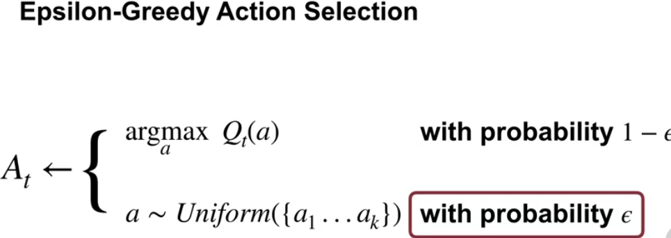
Therefore, we have greedy action selection rule by which the agent always select the acton with the highest estimated value, and epsilon-greedy action selection rule by which the agent behave greedily most of the time, but select randomly among all actions regardless of their estimated action values with a small probability epsilon.
Other methods for balancing exploitation and exploration include optimistic initial values and upper-confidence bound action selection. The former only drive early exploration and are not suited for non-stationary problems. It also require some knowledge of the max reward which is usually set as the optimistic initial value.
-
How is k-armed bandit algorithm used in industry?
K-armed bandit algorithm can be used as alternative for A/B test. In a typical A/B test, traffic is split randomly between variables with equal probability, and the overall payoff achieved equals the average payoff of all the variants, which must be lower than that of the winning variant. That is, A/B tests can have high regret.
Alternatively, k-armed bandit solution uses what’s learned from the experiment to allocate more contacts to variants that perform well and less contacts to variants that are underperforming, therefore producing higher overall payoff and less regret. Depending on the exploration-exploitation strategy, the three most popular k-armed bandit algorithm are Epsilon Greedy, Thompson Sampling and Upper Confidence Bound 1 (UCB-1).
In a typical experimental setup, k-armed bandit method is used to scan a large number of variants to yield an optimized one. Then an A/B test will be running between the control and the new optimized variant to assess the impact and rolling out the winner given the target KPI.
References:
- https://en.wikipedia.org/wiki/Multi-armed_bandit
- https://www.coursera.org/specializations/reinforcement-learning
Note: This article is part of my personal note series of the Reinforcement learning Specialization provided by the Unversity of Alberta and Alberta Machine Intelligence Institute on Coursera.
K-armed Bandit Problem
K-armed bandit problem (or multi-armed bandit problem) is a problem in which a fixed limited set of resources must be allocated between competing or alternative choices in a way that maximize their expected gain, when each choice’s properties are only partially known at the time of allocation.[1] Here the alternative choices are called actions, the gain is called reward, and the one who choose is called agent. The reward each action takes is stochastically choosen from a probability distribution (where uncertainty comes from), and the goal of the agent is to maximize the overall gains at each step. K-armed bandit problem is a sequential decision making process under uncertainty, and a classic reinforcement learning problem that exemplifies the exploration–exploitation tradeoff dilemma.[1]
An example is a doctor (agent) who has to choose between multiple treatments (action) without full knowledge of each treatments’ effect on patients (uncertainty). The doctor’s goal is to maximize the effect (rewards) of the treatments (actions) over some period of time.
If we know the value of each action, then it’s fairly easy to make a choice at each step, as the agent can simply choose the action with the maximum value. However, we don’t know the true value of each action beforehand, therefore we need to estimate the action value through experiments in which the agent takes some action, get rewards, and estimate the action value based on the rewards.
Two major questions can be asked about this process:
-
How to estimate action values? We don’t know the exact value for each action, so we estimate it using sample-average method.
To make the calculation more computationally effective (less memory and less computing power), a bit of mathematical trick can be used so that estimated action value at the current step can be calculated based on the estimated action value and reward from the prior step. This trick is called incremental update rule.
Here 1/n is called step size. It will decay over time as n increases gradually. A more general form of this equation is
The step size can be a constant value between 0 and 1. Is a constant step size better or a decaying step size better? It depends on the specific problem. In general, if the distribution of rewards change over time, i.e., non-stationary bandit problem, using a fixed step size may be more effective. Decay step size may be better for stationary bandit problem of which the distribution of rewards doesn’t change over time.
If a fixed step size is used, the incremental update rule can be further simplified and it’s intuitive that contribution from past rewards (n-t) decay exponentially with distance to the present time step (t).
Choosing a fixed step size also requires experimentation. If the step size is too small, the estimated action value may not get close to the actual value; if it is too big, the estimated value may be very susceptible to stochasticity in the rewards and thus oscillate around the true value too much.
Keep in mind that due to the uncertainty in such experiments, a large number of runs (i.e., hundreds) are required and their averaged values are needed in order to fairly compare the impact of step sizes.
-
Based on what principles does the agent take action during the experiments?
Even if the agent knows the estimated action values at each step, it may take different actions. It can simply choose the action with the highest estimated value, or randomly choose an action regardless of its action value. The former is called exploitation and the later is called exploration. Exploitation will help the agent maximize short term rewards based on partial knowledge, and thus the agent may lose the opportunity to explore other actions and optimize overall returns in the long run. Exploration allows the agent to know more about all actions and thus optimize overall returns in the long run, however, the short-term return may not be optimal.
Therefore, we have greedy action selection rule by which the agent always select the acton with the highest estimated value, and epsilon-greedy action selection rule by which the agent behave greedily most of the time, but select randomly among all actions regardless of their estimated action values with a small probability epsilon.
Other methods for balancing exploitation and exploration include optimistic initial values and upper-confidence bound action selection. The former only drive early exploration and are not suited for non-stationary problems. It also require some knowledge of the max reward which is usually set as the optimistic initial value.
-
How is k-armed bandit algorithm used in industry?
K-armed bandit algorithm can be used as alternative for A/B test. In a typical A/B test, traffic is split randomly between variables with equal probability, and the overall payoff achieved equals the average payoff of all the variants, which must be lower than that of the winning variant. That is, A/B tests can have high regret.
Alternatively, k-armed bandit solution uses what’s learned from the experiment to allocate more contacts to variants that perform well and less contacts to variants that are underperforming, therefore producing higher overall payoff and less regret. Depending on the exploration-exploitation strategy, the three most popular k-armed bandit algorithm are Epsilon Greedy, Thompson Sampling and Upper Confidence Bound 1 (UCB-1).
In a typical experimental setup, k-armed bandit method is used to scan a large number of variants to yield an optimized one. Then an A/B test will be running between the control and the new optimized variant to assess the impact and rolling out the winner given the target KPI.
References:
- https://en.wikipedia.org/wiki/Multi-armed_bandit
- https://www.coursera.org/specializations/reinforcement-learning
Note: This article is part of my personal note series of the Reinforcement learning Specialization provided by the Unversity of Alberta and Alberta Machine Intelligence Institute on Coursera.
Comments
Join the discussion for this article on this ticket. Comments appear on this page instantly.