Reinforcement Learning Series Overview
This article series include my personal notes of the Reinforcement learning Specialization provided by the Unversity of Alberta and Alberta Machine Intelligence Institute on Coursera. The following four courses covered in this specialization are:
-
- Foundamentals of Reinforcement Learning
- 1.1 K-armed bandit problem
- 1.2 Markov decision processes
- 1.3 Value functions and Bellman equations
- 1.4 Policy Iteration and Dynamic Programming
-
- Sample-based Learning Methods
-
- Prediction and Control with Function Approximation
Week 2, Markov decision processes (MDP) and goal of agent in reinforcement learning
Week 3, Value functions and Bellman equations
Now we have formally defined the MDPs and goal of reinforcement learning, our next question comes naturally – how do we calculate the rewards for any MDPs and decide on the optimal way to act in order to maximize expected returns?
We need to be quantitative here. So let’s first define some quantities using some mathematical formula, and translate our initial question into an optimization problem.
-
Policy
A policy is a mapping from states to probabilities of selecting each possible action. It tells an agent how to behave in their environment. If an agent is folloiwng a policy Pi at time t, then Pi(a
s) is the probability that At = a if St = s. If Pi is a constant for every single state, meaning there is only one action to take after each state, this policy is called a deterministic policy. Otherwise, it is called a stochastic policy. For stochastic policy, the following condition is satisfied:
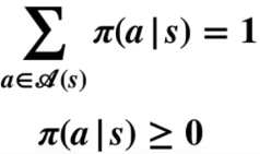
For MDPs (note most reinforcement learning process constitutes a MDP), policies are only determined by the current state, not other things like time or previous states.
-
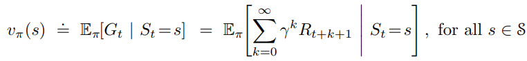
Value function
A value function defines the expected return for a state or state-action pair. Specifically, a state-value function of a state s under policy Pi is defined as:
An action-value function of taking action a in state s under a policy Pi is defined as:
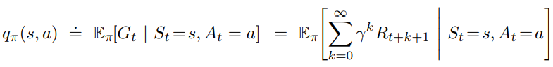
Note that both value functions quantify the expected return at a certain state, so the state-value function is a collective sum of action-value functions over different actions at the same state.
-
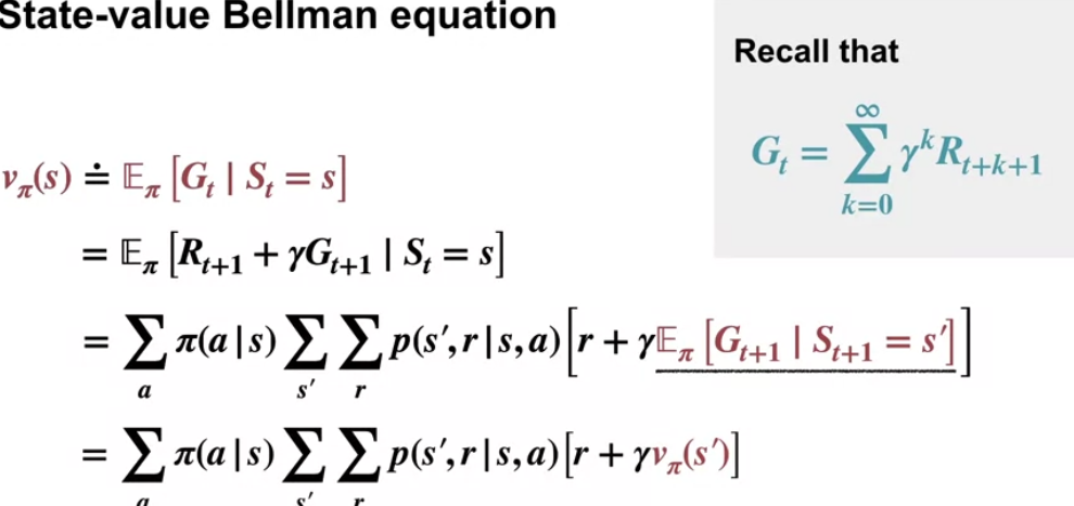
Bellman equation
Bellman equation denotes the relationship between value functions of the present state and value functions of its possible successor state. With Bellman equations and some termination conditions, value function for each state and state-action pairs can be calculated.

A good example of using Bellman equation to calculate value function is Gridworld (see Page 60 of the textbook).
Now we know how to calculate expected return of each state, so what is considered an optimal policy which can guarantee the maximum return? Formally, an optimal policy is defined as a policy that is at least as good (has the same or higher state-value function) as every other policy in every state. A finite MDP may have more than one optimal policy but they will all share the same value function.
Under optimal policy, optimal functions are defined as follows:

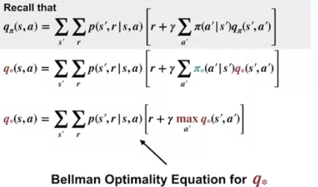
Similarly, Bellman optimality equations can be used to calculate optimal value functions under optimal policy. If we have the optimal state-value function or optimal action-value function, it is easy to work out the optimal policy.
Week 4, Policy Iteration and Dynamic Programming
Now we know by solving Bellman equation state-value function and action-value function can be calculated – the prediction problem. If we have the optimal state-value function or optimal action-value function, we can easily find out the optimal policy. So the question is how do we find optimal state-value function or optimal action-value function based on randomly initialized values given that value functions are usually randomly initialized because we have little knowledge about them?
The process of finding an optimal policy — the control problem — is called policy iteration. Dynamic programming is the computation method used for updating the values in this optimization process.
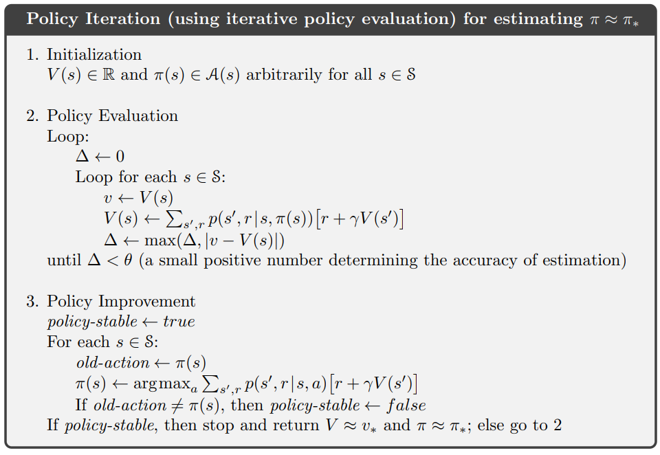
Policy Iteration
Policy iteration contains three major steps as follows:
-
Initializing state-value function and policy arbitrarily for all states and actions involved. This step is easy as both state-value function and policy are represented as matrixes and we all know how to randomly initialize them. For example, a system has m states and n actions in each state, then the state-value function will be a m x 1 matrix and the policy will be an m x n matrix.
-
Policy evaluation. It is the task of determining state-value function V for a policy Pi using Bellman equation. The state-value functions are updated iteratively using dynamic programming until the values converge (doesn’t change much anymore.)
-
Policy improvement. It is the process of making a new policy that improves on an original policy, by making it greedy with respect to the state-action value function of the original policy. Here greedy means choosing the action at the current state to be the one with the maximum state-action value among all actions, then update the policy accordingly.
Below is a toy implementation of this process in Python.
def policy_iteration(env, gamma, theta):

    # 1. initialization of state value function V and policy pi
    V = np.zeros(len(env.S))
    pi = np.ones((len(env.S), len(env.A))) / len(env.A)
    policy_stable = False

    while not policy_stable:

        # 2. policy evaluation
        V = evaluate_policy(env, V, pi, gamma, theta)

        # 3. policy improvement
        pi, policy_stable = improve_policy(env, V, pi, gamma)

    return V, pi

def evaluate_policy(env, V, pi, gamma, theta):
    delta = float('inf')
    while delta > theta:
        delta = 0
        for s in env.S:
            v = V[s]

            # Bellman update
            new = 0
            for action in range(len(pi[0])):
                transitions = env.transitions(s, action)
                for state in range(len(transitions)):
                    reward = transitions[state][0]
                    p = transitions[state][1]
                    new += pi[s][action]*p*(reward + gamma*V[state])
            V[s] = new

            delta = max(delta, abs(v - V[s]))

    return V


def improve_policy(env, V, pi, gamma):
    policy_stable = True
    for s in env.S:
        old = pi[s].copy()

        # q greedify policy
        num_actions = len(pi[0])
        q = [0 for _ in range(num_actions)]
        for action in range(num_actions):
            transitions = env.transitions(s, action)
            for state in range(len(transitions)):
                reward = transitions[state][0]
                p = transitions[state][1]
                q[action] += p*(reward + gamma*V[state])
        max_action = np.argmax(q)
        pi[s] = [0 if i != max_action else 1 for i in range(num_actions)]

        if not np.array_equal(pi[s], old):
            policy_stable = False

    return pi, policy_stable
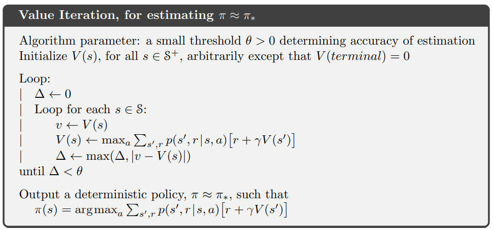
One question we may ask here is that there are much overlapped computation between the policy evaluation and policy improvement step, so it it possible to simplify such process? The answer is Yes, by truncating the policy evaluation step to only one sweep (one update of each state). Convergence to the optimal policy is proved to be still guaranteed. This algorithm is called value iteration. See detailed implementation below.
def value_iteration(env, gamma, theta):
    V = np.zeros(len(env.S))

    while True:
        delta = 0
        for s in env.S:
            v = V[s]

            # Bellman Optimality update
            num_actions = len(pi[0])
            q = [0 for _ in range(num_actions)]
            for action in range(num_actions):
                transitions = env.transitions(s, action)
                for state in range(len(transitions)):
                    reward = transitions[state][0]
                    p = transitions[state][1]
                    q[action] += p*(reward + gamma*V[state])
            V[s] = max(q)

            delta = max(delta, abs(v - V[s]))
        if delta < theta:
            break

    # policy update
    pi = np.ones((len(env.S), len(env.A)))/len(env.A)
    for s in env.S:
        # q greedify policy
        num_actions = len(pi[0])
        q = [0 for _ in range(num_actions)]
        for action in range(num_actions):
            transitions = env.transitions(s, action)
            for state in range(len(transitions)):
                reward = transitions[state][0]
                p = transitions[state][1]
                q[action] += p*(reward + gamma*V[state])
        max_action = np.argmax(q)
        pi[s] = [0 if i != max_action else 1 for i in range(num_actions)]

    return V, pi
Dynamic programming
Dynamic programming (DP) is a general approach to solving problems by breaking them into subproblems that can be solved separately, cached, then combined to solve the overall problem. It can be used to solve both policy evaluation and control tasks in MDP, if we have access to the dynamics function p. The reason we need dynamic programming in reinforcement learning is because it is computationally more efficient than other methods such as Monte Carlo Sampling or Brutal-force Search. DP is synchronous if it systematically sweeps the entire state space at each iteration (update every state exactly once at each iteration) and aynchronous if it does not update all states at each iteration and updates some states more than others. Asynchronous DP converges faster than synchornous DP and thus used widely in real world reinforcement learning problem.
Reinforcement Learning Series Overview
This article series include my personal notes of the Reinforcement learning Specialization provided by the Unversity of Alberta and Alberta Machine Intelligence Institute on Coursera. The following four courses covered in this specialization are:
-
- Foundamentals of Reinforcement Learning
- 1.1 K-armed bandit problem
- 1.2 Markov decision processes
- 1.3 Value functions and Bellman equations
- 1.4 Policy Iteration and Dynamic Programming
- Foundamentals of Reinforcement Learning
-
- Sample-based Learning Methods
-
- Prediction and Control with Function Approximation
Week 2, Markov decision processes (MDP) and goal of agent in reinforcement learning
Week 3, Value functions and Bellman equations
Now we have formally defined the MDPs and goal of reinforcement learning, our next question comes naturally – how do we calculate the rewards for any MDPs and decide on the optimal way to act in order to maximize expected returns?
We need to be quantitative here. So let’s first define some quantities using some mathematical formula, and translate our initial question into an optimization problem.
-
Policy
A policy is a mapping from states to probabilities of selecting each possible action. It tells an agent how to behave in their environment. If an agent is folloiwng a policy Pi at time t, then Pi(a s) is the probability that At = a if St = s. If Pi is a constant for every single state, meaning there is only one action to take after each state, this policy is called a deterministic policy. Otherwise, it is called a stochastic policy. For stochastic policy, the following condition is satisfied: For MDPs (note most reinforcement learning process constitutes a MDP), policies are only determined by the current state, not other things like time or previous states.
-
Value function
A value function defines the expected return for a state or state-action pair. Specifically, a state-value function of a state s under policy Pi is defined as:
An action-value function of taking action a in state s under a policy Pi is defined as:
Note that both value functions quantify the expected return at a certain state, so the state-value function is a collective sum of action-value functions over different actions at the same state.
-
Bellman equation
Bellman equation denotes the relationship between value functions of the present state and value functions of its possible successor state. With Bellman equations and some termination conditions, value function for each state and state-action pairs can be calculated.
A good example of using Bellman equation to calculate value function is Gridworld (see Page 60 of the textbook).
Now we know how to calculate expected return of each state, so what is considered an optimal policy which can guarantee the maximum return? Formally, an optimal policy is defined as a policy that is at least as good (has the same or higher state-value function) as every other policy in every state. A finite MDP may have more than one optimal policy but they will all share the same value function.
Under optimal policy, optimal functions are defined as follows:
Similarly, Bellman optimality equations can be used to calculate optimal value functions under optimal policy. If we have the optimal state-value function or optimal action-value function, it is easy to work out the optimal policy.
Week 4, Policy Iteration and Dynamic Programming
Now we know by solving Bellman equation state-value function and action-value function can be calculated – the prediction problem. If we have the optimal state-value function or optimal action-value function, we can easily find out the optimal policy. So the question is how do we find optimal state-value function or optimal action-value function based on randomly initialized values given that value functions are usually randomly initialized because we have little knowledge about them?
The process of finding an optimal policy — the control problem — is called policy iteration. Dynamic programming is the computation method used for updating the values in this optimization process.
Policy Iteration
Policy iteration contains three major steps as follows:
-
Initializing state-value function and policy arbitrarily for all states and actions involved. This step is easy as both state-value function and policy are represented as matrixes and we all know how to randomly initialize them. For example, a system has m states and n actions in each state, then the state-value function will be a m x 1 matrix and the policy will be an m x n matrix.
-
Policy evaluation. It is the task of determining state-value function V for a policy Pi using Bellman equation. The state-value functions are updated iteratively using dynamic programming until the values converge (doesn’t change much anymore.)
-
Policy improvement. It is the process of making a new policy that improves on an original policy, by making it greedy with respect to the state-action value function of the original policy. Here greedy means choosing the action at the current state to be the one with the maximum state-action value among all actions, then update the policy accordingly.
Below is a toy implementation of this process in Python.
def policy_iteration(env, gamma, theta):
# 1. initialization of state value function V and policy pi
V = np.zeros(len(env.S))
pi = np.ones((len(env.S), len(env.A))) / len(env.A)
policy_stable = False
while not policy_stable:
# 2. policy evaluation
V = evaluate_policy(env, V, pi, gamma, theta)
# 3. policy improvement
pi, policy_stable = improve_policy(env, V, pi, gamma)
return V, pi
def evaluate_policy(env, V, pi, gamma, theta):
delta = float('inf')
while delta > theta:
delta = 0
for s in env.S:
v = V[s]
# Bellman update
new = 0
for action in range(len(pi[0])):
transitions = env.transitions(s, action)
for state in range(len(transitions)):
reward = transitions[state][0]
p = transitions[state][1]
new += pi[s][action]*p*(reward + gamma*V[state])
V[s] = new
delta = max(delta, abs(v - V[s]))
return V
def improve_policy(env, V, pi, gamma):
policy_stable = True
for s in env.S:
old = pi[s].copy()
# q greedify policy
num_actions = len(pi[0])
q = [0 for _ in range(num_actions)]
for action in range(num_actions):
transitions = env.transitions(s, action)
for state in range(len(transitions)):
reward = transitions[state][0]
p = transitions[state][1]
q[action] += p*(reward + gamma*V[state])
max_action = np.argmax(q)
pi[s] = [0 if i != max_action else 1 for i in range(num_actions)]
if not np.array_equal(pi[s], old):
policy_stable = False
return pi, policy_stable
One question we may ask here is that there are much overlapped computation between the policy evaluation and policy improvement step, so it it possible to simplify such process? The answer is Yes, by truncating the policy evaluation step to only one sweep (one update of each state). Convergence to the optimal policy is proved to be still guaranteed. This algorithm is called value iteration. See detailed implementation below.
def value_iteration(env, gamma, theta):
V = np.zeros(len(env.S))
while True:
delta = 0
for s in env.S:
v = V[s]
# Bellman Optimality update
num_actions = len(pi[0])
q = [0 for _ in range(num_actions)]
for action in range(num_actions):
transitions = env.transitions(s, action)
for state in range(len(transitions)):
reward = transitions[state][0]
p = transitions[state][1]
q[action] += p*(reward + gamma*V[state])
V[s] = max(q)
delta = max(delta, abs(v - V[s]))
if delta < theta:
break
# policy update
pi = np.ones((len(env.S), len(env.A)))/len(env.A)
for s in env.S:
# q greedify policy
num_actions = len(pi[0])
q = [0 for _ in range(num_actions)]
for action in range(num_actions):
transitions = env.transitions(s, action)
for state in range(len(transitions)):
reward = transitions[state][0]
p = transitions[state][1]
q[action] += p*(reward + gamma*V[state])
max_action = np.argmax(q)
pi[s] = [0 if i != max_action else 1 for i in range(num_actions)]
return V, pi
Dynamic programming
Dynamic programming (DP) is a general approach to solving problems by breaking them into subproblems that can be solved separately, cached, then combined to solve the overall problem. It can be used to solve both policy evaluation and control tasks in MDP, if we have access to the dynamics function p. The reason we need dynamic programming in reinforcement learning is because it is computationally more efficient than other methods such as Monte Carlo Sampling or Brutal-force Search. DP is synchronous if it systematically sweeps the entire state space at each iteration (update every state exactly once at each iteration) and aynchronous if it does not update all states at each iteration and updates some states more than others. Asynchronous DP converges faster than synchornous DP and thus used widely in real world reinforcement learning problem.
Comments
Join the discussion for this article on this ticket. Comments appear on this page instantly.